Vector Autoregressive (VAR) Models with R : relationship between the S&P500, Bitcoin, CHF, JPY
- idriss tsafack

- Feb 2, 2021
- 9 min read
Updated: Dec 6, 2021
Hey there! Welcome back to my blog! In this post I will show you how to estimate the Vector Autoregressive (VAR) model with R.
Feel free to contact me for any consultancy opportunity in the context of big data, forecasting, and prediction model development (idrisstsafack2@gmail.com) .

This post in in the continuity of my post series related to time series analysis. If it's your first time to be here, I suggest that you check also my other posts. Indeed, you can check my post on ARMA model with R titled " "ARMA models with R: the ultimate practical guide with Bitcoin data " or my previous post on GARCH models with R titled "GARCH models with R programming : a practical example with TESLA stock ". In those post I show you the rationale behind those time series models.
When observing ARMA and GARCH models, you can immediately notice that estimations and forecasting are done on one single variable. In real life, this does not hold. Indeed, there are many other variables that could influence the other variables. For example on the financial markets, when the stock market is selling-off, usually market participant tend to hedge their position by buying more gold, assets labelled in Japanese Yen (JPY) currency or Swiss Franc (CHF) currency, and potentially Bitcoin. There exist another class of asset used to hedge long term position such as countries bond assets and insurance products or options.
Then market participants and economist are always interested in the dynamic relationship between macroeconomic variables and the assets they are interested to buy. This operation can help them anticipate the potential scenario that can happen on the market.
This means that usually there exist other variables that can affect the dynamics of the variable of interest. VAR models for time series are well adapted to the context where we would like to identify the short term relationship between two or more time series variables. Also if we would like to analyze the impact of the shock of a variable on another variable. One popular example in economics is the diagnostic of the impact of central back interest rate on GDP or on a given currency.
The purpose of this article is to present the model setting of the VAR models and to show how to estimate those models with R. In the first section I will talk about the setting of the model and in the second part I will go straight to the practical example. For the example, we will not use Game Stop but I will consider 4 financial variables that are : S&P 500, Bitcoin, JPY currency and CHF currency.
VAR Models setting
To explain the VAR model setting, I will use a simple illustration. Imagine that you are an amazon seller and you have 2 products in your store : banana and orange. Based on your analysis you observe that there is a sort of correlation between the sales volume of banana and the one of oranges. You would like to know an increase in banana sales can impact orange sales. On the same line, orange sales can also impact banana sales. Then, we can have a reverse causality between the two variables. Then a VAR model consider both sense of causality of the variables and analyze the relationship between the sales in banana and sales in orange.
The basic Vector Autoregressive model of order "1" named VAR(1) with the considered variables is presented as follows :

The setting presented means that the orange sales volumes depends on previous period sales and the previous sales recorded in banana. The number of lags considered in this model is one. Similar to what we observed from the ARMA or GARCH models one should select the optimal number of lag to consider for the model.
Then, for a generalization, let Y_t = (Y_1t,...,Y_nt)' denote an (n by 1) vector of time series variables (Each variable Y_it contains a number T of observation of the time series). The basic Vector Autoregressive model of order "p" named VAR(p) is presented as follows :

"p" is the number of lag considered in the model. Based on this model setting we can define the invariant covariance matrix of the error term.
Model Estimation
We can recast the model and stack the data for each variable considered considered as a response variable.

Selection of the number of lag for the model
There exist 2 main approaches to select the number of lag for the model :
The empirical approach, where we use an information criterion
The inference approach which consist in using hypothesis testing
For this post, we consider only the information criteria. There are 3 popular information criteria, that are :
Akaike Information Criterion (AIC)
Schwarz-Bayesian (BIC)
Hannan-Quinn (HQ)
Indeed, the optimal number of lag is the one such that the information criterion is minimal. Then, we estimate the VAR(p) for p= 0,...,pmax and choose the value p that minimizes the AIC, BIC or HIQ.
Here are the following formula of the considered criteria

For more details about the algebra related to this model, check the book by Hamilton (1985)
Real data Applications
In this section, we will present an application on the financial market. In this application, we will try to model the dynamic relationship between the SP500, Bitcoin currency , JPY currency and CHF currency. The idea is to see if the stock market crash can lead to bitcoin increase. Another question is to see which of the the currency is more considered by market participant.
The first step of the operation is to load the packages necessary for the estimations
The first step of the operation is to load the packages necessary for the estimationsc, that are : "quantmod" for financial data scraping, "vars" for VAR model specification and estimation, "xts" for time series manipulation and "PerformanceAnalytics" to analyze the performance of our models setting. Here is the related code.

Once we have loaded the different packages, we can get the symbol of the variables of interest, that are Bitcoin, JPY, CHF, SP500. To get the TSLA data, we use the function getSymbols(). Here is the code. We consider the daily data from January 2015 to December 2015.

Now we can display the different time series of variables.
Bitcoin currency

JPY Currency

CHF Currency

SP500

For the VAR estimation, we will consider the time series from January to December 2020 at the daily frequency. Here is the code for transforming the data frame into time series variables

Once we have the time series, we can calculate the daily returns for each variable. For the return calculation we use the function CalculateReturns(). Then we have the following code.

We use again the function chartSeries() in order to display the time series of the returns. Here is the graph of the returns for the different variables.
SP500 returns

JPY currency

BTC currency

CHF currency

Based on the figures of the returns, we can see that we have their variances change with time, meaning that we can suspect the time series are nonstationary. The next step is to check the autocorrelation function and the partial autocorrelation function. Here is the code

We obtain the following graphs
ACF and PACF for Bitcoins


ACF and PACF for JPY Currency


ACF and PACF for CHF Currency


ACF and PACF for SP500


Based on the ACF and PACF we can notice that for each variable we should consider at least 3 lags for the model setting. We will check if this is the case in the econometric analysis.
P.S.: Feel free to contact me for any consultancy opportunity in the context of big data, forecasting, and prediction model development (idrisstsafack2@gmail.com).
Now, for the model estimation, we need to pool the 4 variables all together on the same data frame. Also, we should select the optimal number of lags for the model estimation. The function for a number of lag selection is called VARselect(). The optimal number of lag considered for the model setting is equal to 5.

The function used for the model estimation is called VAR(). We use the summary() function to see the results of the estimations. We kept the estimations very basic and simple, meaning that we didn't considered the seasonality effect of variables. Also we didn't considered the additional exogenous variables that could be used as control variables in the estimation procedure.

The function summary() will provide the results of the estimations. Indeed, we obtain 4 tables. Each table represent the OLS estimation projecting one of the 4 considered variables onto the three others. Here are the tables of results. The first table shows the projection of SP500 onto BTC, JPY and CHF and their relative lags. For each variable we consider the 5 previous lags in the regression. The other tables are presented on the same fashions with the other variables.


From the third table, we can see that the SP500, BTC and JPY tends to significantly impact the the CHF currency. This model is still very fallacious as we do not consider the seasonality , the jumps and the other macroeconomic variables that can affect the variables.


The last table show the matrix of covariances and the matrix of correlations. We can observe that the CHF currency is highly negatively correlated with JPY. Also, CHF currency is negatively correlated with BTC and SP500

Performance evaluation of the model
For the performance evaluation of the model, we run 4 different tests :
The test of the presence of serial correlation in the residuals : serial.test()
The heteroskedasticity test : arch.test()
The normality test of the residuals : normality.test()
The presence of structural break in the residuals : stability()
Here are the related code

We obtain the following results. The first test relative to the presence of serial correlation in the residual also called the Portmanteau Test, we can see that the p-value of the test is close to zero, meaning that we reject the null hypothesis of nonexistence of serial correlations. Then, we should consider the serial correlation of residuals
Concerning the test of heteroskedasticity, we can see that the p-value is equal to 1, meaning that we accept the null hypothesis meaning that we have the presence of the heteroskedasticity in the residuals
The Jarque Bera test is then used to check if the residuals fit the normal distribution. From the test we can see that the p-value is higher than 0.05, meaning thatthe residuals tend to fit the normal distribution.

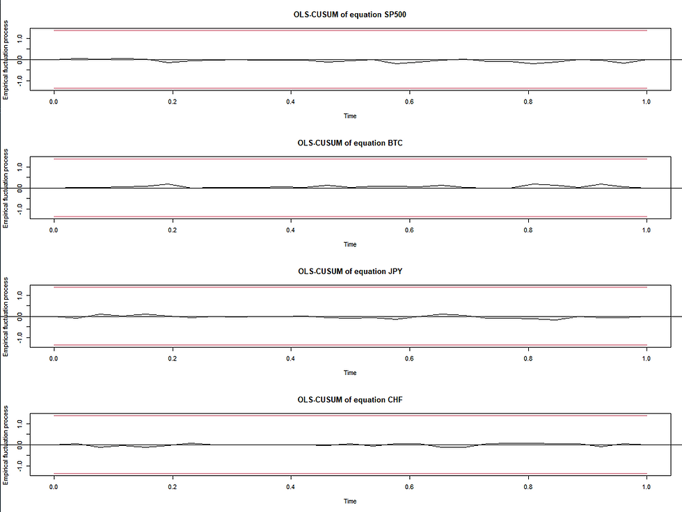
The last test consider checking the presence of structural breaks in the residuals. We can see on the figure below that for each variable, we can see that the empirical process of residual stay in the confidence intervals, meaning that there is no structural break.
Granger causality
When running the VAR model, one of the most important test that we would like to check is the causality test. The idea of the causality is to check is the presence of a certain variable contribute to forecast another variable. The function used for the test is called causality(). The Granger causality test is the most used for that purpose. Here is the code for the Granger test and the related results.
For example, when we test if JPY Granger causes SP500, BTC and CHF, we use the function causality(). The p-value of the test is close to zero (lower than 5%) meaning we reject the null hypothesis. Hence, the JPY Granger causes BTC, SP500 and CHF. The JPY currency contributes to the prediction of the other variables. We can also observe that JPY currency instantaneously causes the other variables. We obtain the same result when checking the results of the test for other variables of the model.


Impulse response function
The impulse response function is usually used to check how certain variables behave to a random chock on a considered variable. For example we can be interested in how BTC, CHF, and JPY can react to a chock on the stock market. Then, we use the impulse response function. The code used to calculate the impulse response function object for each variable is called irf().
Here bellow, we present the results of the reaction of BTC, CHF and JPY on a chock from the SP500. The effect are evaluated for a period of 20 days.

We obtain the following plot. We can see that a chock on the SP500 leads to a decrease of the value of JPY, an increase of the value of CHF and an increase of BTC on the next 20 days. This effect is more pronounced on the last 10 days.
Impact on JPY

Impact on CHF

Impact on BTC

Forecasting
Now, we can forecast the considered variables. To forecast the variables 20 day ahead, we use the function predict(). Then, the code is presented as follows.

The forecast are presented as follows. As we can see, after December 2020, we expect the JPY to decrease on the next 20 days. For the same period considered, we expect the SP500, BTC and CHF currency to increase.


References :
1. Bollerslev, T., Chou, R. Y., and Kroner, K. F. (1992) ARCH modelling in finance. Journal of Econometrics, 52, 5–59.
2. Bollerslev, T., Engle, R. F., and Nelson, D. B. (1994) ARCH models, In Handbook of Econometrics, Vol IV, Engle, R.F., and McFadden, D.L., Elsevier, Amsterdam
3. Gourieroux, C. and Jasiak, J. (2001) Financial Econometrics, Princeton University Press, Princeton, NJ.
4. Hamilton, J. D. (1994) Time Series Analysis, Princeton University Press, Princeton, NJ.


Comments